The Anatomy of an ODE solver: Implementing Euler and Runge-Kutta in Common Lisp

2026-07-06 differential-equations

Lately, I've been working on a paper where I optimize some continuous parameters of a flying robot in a hummingbird robot with MuJoCo MJX. One of the early problems I faced was that no learned design transferred to other integrators or timesteps than the one that it was trained on. This means that the gradient descent simply learned the quirks of the numerical scheme rather than any meaningful physics.

When learning over physics simulators, it is probably best to have at least a basic understanding of numerical analysis and solving ODEs so you know how the Physics simulator actually works. In this post, I will cover the basics of IVPs and methods for solving, specifically Euler and RK4. Ultimately, we will solve the Euler-Lagrange equation to compute the forward dynamics of an ideal pendulum.

The Foundations

What kind of ODEs are we solving? Where are they useful? What is the simplest method of solving them?

Initial Value Problems (IVPs)

An IVP is the function we're solving for, pinned down by two things:

\begin{equation*} \underbrace{y'(t) = f(t, y(t))}_{\text{the rule for change}} \end{equation*}

\begin{equation*} \underbrace{y(t_0) = y_0}_{\text{where we start}} \end{equation*}

The function $f(t, y(t))$ is the vector field. Given the time and current position, it will return the rate of change at that time.

$y(t)$ also need not be a scalar. It is a vector valued function $y(t) \in \mathbb{R}^d$ where $d$ can be 1 or 1000.

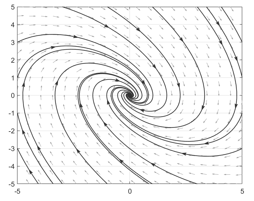
The entire point of numerical analysis can be stated intuitively as trying to find the function $y(t)$ outlined by some vector field $f(t, y(t))$.

Aside: Physics simulation as an IVP

This relatively simple class of problems can abstract a wide range of physical phenomena. In fact, classical mechanics itself can be formulated as an IVP, which is almost exactly what many conventional physics simulators actually do. Lets formalize this.

Euler-Lagrange gives you a second-order ODE

\begin{equation*} \frac{d}{dt} \left( \frac{\partial L}{\partial \dot{q}} \right) - \frac{\partial L}{\partial q} = \tau \end{equation*}

This is an order 2 ODE. The order is determined by the highest derivative of the dependent variable in the equation. Euler and RK4 are meant to solve first order problems.

Make the accelerations explicit

The Lagrangian is defined as $$L = \frac{1}{2} \dot{q}^T m(q) \dot{q} - V(q)$$. By computing the derivatives and rewriting the Euler-Lagrange equation, we receive the manipulator equation:

\begin{equation*} M(q)\ddot{q} + C(q, \dot{q})\dot{q} + g(q) = \tau \end{equation*}

We can solve for acceleration by doing: $\ddot{q} = M(q)^{-1}[\tau - (C(q, \dot{q})\dot{q} - g(q))]$

Collapse second-order into first-order

Euler and RK are built for $y' = f(t, y)$, first order. To reconcile this, we can double the state: $x = \begin{pmatrix} q \\ \dot{q} \end{pmatrix} \in \mathbb{R}^{2n}$

$\dot{x} = \frac{d}{dt} \begin{pmatrix} q \\ \dot{q} \end{pmatrix} = \begin{pmatrix} \dot{q} \\ \ddot{q} \end{pmatrix} = \begin{pmatrix} \dot{q} \\ M(q)^{-1} [\tau - C(q, \dot{q})\dot{q} - g(q)] \end{pmatrix}$

Given an initial condition, this becomes exactly an IVP.

\begin{equation*} x(t_0) = \begin{pmatrix} q_0 \\ \dot{q}_0 \end{pmatrix} \end{equation*}

Later in this post, we will write the equations for a pendulum in this way.

Our Goal: IVP for a pendulum

The IVP that we will solve is for the following problem. For a simple pendulum: a point mass $m$ on a massless rod of length l, with angle $\theta$ measured from the downward vertical.

\begin{equation*} L = \frac{1}{2}ml^2 \dot{\theta}^2 - mgl(1-\cos\theta) \end{equation*}

After applying Euler lagrange, we get:

\begin{align*} \frac{\partial L}{\partial \theta} &= -mgl\sin(\theta) \\ \frac{\partial L}{\partial \dot{\theta}} &= ml^2\dot{\theta} \\ \frac{d}{dt} \left(\frac{\partial L}{\partial \dot{\theta}}\right) &= ml^2\ddot{\theta} \end{align*}

The final ODE is:

\begin{equation*} ml^2\ddot{\theta} - mgl\sin\theta = 0 \end{equation*}

If we rewrite it as a first order ODE:

\begin{align*} \dot{\theta} &= \omega \\ \dot{\omega} &= - \frac{g}{l} \sin \theta \end{align*}

Now lets rewrite it as a state vector:

\begin{align*} x &= \begin{bmatrix} \theta \\ \omega \end{bmatrix} \\ \dot{x} &= \begin{bmatrix} \dot{\theta} \\ \dot{\omega} \end{bmatrix} = \begin{bmatrix} \omega \\ -\frac{g}{l} \sin\theta \end{bmatrix} \end{align*}

Euler's Method

The flow for a numerical method looks something like this. You start at some point $y_0$. Then, you take the derivative formula, but refuse to take the limit.

\begin{equation*} y'(t) \approx \frac{y(t+h)-y(t)}{h} \Rightarrow y(t+h) \approx y(t) + h y'(t) = y(t) + h f(t, y(t)) \end{equation*}

This gives us the equation for the value of the function at a short timestep away, where accuracy is inversely correlated with the size of the timestep.

\begin{align*} t_{n+1} &= t_n + h, \\ y_{n+1} &= y_n + h f(t_n, y_n) \end{align*}

With Euler's method, the simplest possible method, we receive the following recurrence.

Error and Order

For a given method, we need to evaluate how faithfully it follows the true solution. Any method that requires an extremely small timestep to keep a low error quickly becomes computationally expensive.

Local Truncation Error (LTE)

Local truncation error is the difference between the approximated value at the next timestep vs the real value. It is local to the next timestep, meaning the global error compounds.

$T_{n+1} = y(n+1) - \left[y_n + h y'(n)\right]$

Computing Euler's LTE

If you model Euler method as a first order taylor series, the remaining (order 2 and beyond) components of the Taylor series are the true error. Because the dominating term in the error of the Taylor series is the $h^2$ term, we can say that the error is proportional to $h^2$. $y(n+h) = y_n + h y'(n) + \frac{h^2}{2} y''(n) \dots$

The order $p$ of the method is just $h^{1 + p}$, where $1 + p$ is the exponent of the dominating term of the error. Hence, Euler is an order 1 method.

Local vs global

$\text{number of steps} = \frac{T-t_0}{h} \propto \frac{1}{h}$

Global error can be found by accumulating the error at each step, and multiplying it by the number of steps: $\frac{1}{h} \times h^2 = h$

Euler in Common Lisp

First, we define some common vectorization functions, to make Lisp lists act like Numpy arrays:

(defun map-functions (functions scalars)
  "Apply each function in FUNCTIONS to the corresponding scalar in SCALARS."
  (mapcar #'funcall functions scalars))

(defun vec-add (a b)
  "Element-wise addition of two lists."
  (mapcar #'+ a b))

(defun vec-scale (scalar scalars)
  "Multiply each element of SCALARS by SCALAR."
  (mapcar (lambda (x) (* scalar x)) scalars))

Next, we define the IVP struct, and formulate the pendulum as an IVP. Notice how the ODE is treated as a single, vector valued function. It takes the full state as input, and outputs a list of functions (which rely on that full state) as output.

(defstruct ivp
  ode
  initial-state)

(defstruct pendulum-params
  (length 1.0)
  (g 9.81))

(defun make-pendulum-ode (params)
  (lambda (state)
    (let ((theta (first state))
          (omega (second state))
          (l (pendulum-params-length params))
          (g (pendulum-params-g params)))
      (list omega (- (* (/ g l) (sin theta)))))))

(defun make-pendulum-ivp (&key (theta0 0.5) (omega0 0.0) (length 1.0) (g 9.81))
  (make-ivp
   :ode (make-pendulum-ode (make-pendulum-params :length length :g g))
   :initial-state (list theta0 omega0)))

And the Euler solver itself:

(defun euler-step (timestep ivpair)
  (let* ((state (ivp-initial-state ivpair))
         (derivs (funcall (ivp-ode ivpair) state))
         (new-ivp (copy-ivp ivpair))
         (inc (vec-scale timestep derivs)))
    (setf (ivp-initial-state new-ivp) (vec-add state inc))
    new-ivp))

(defun euler-solve (timestep ivpair time)
  (let ((num-timesteps (floor (/ time timestep))))
    (loop for i from 0 to num-timesteps
          for current = ivpair then (euler-step timestep current)
          collect (ivp-initial-state current))))

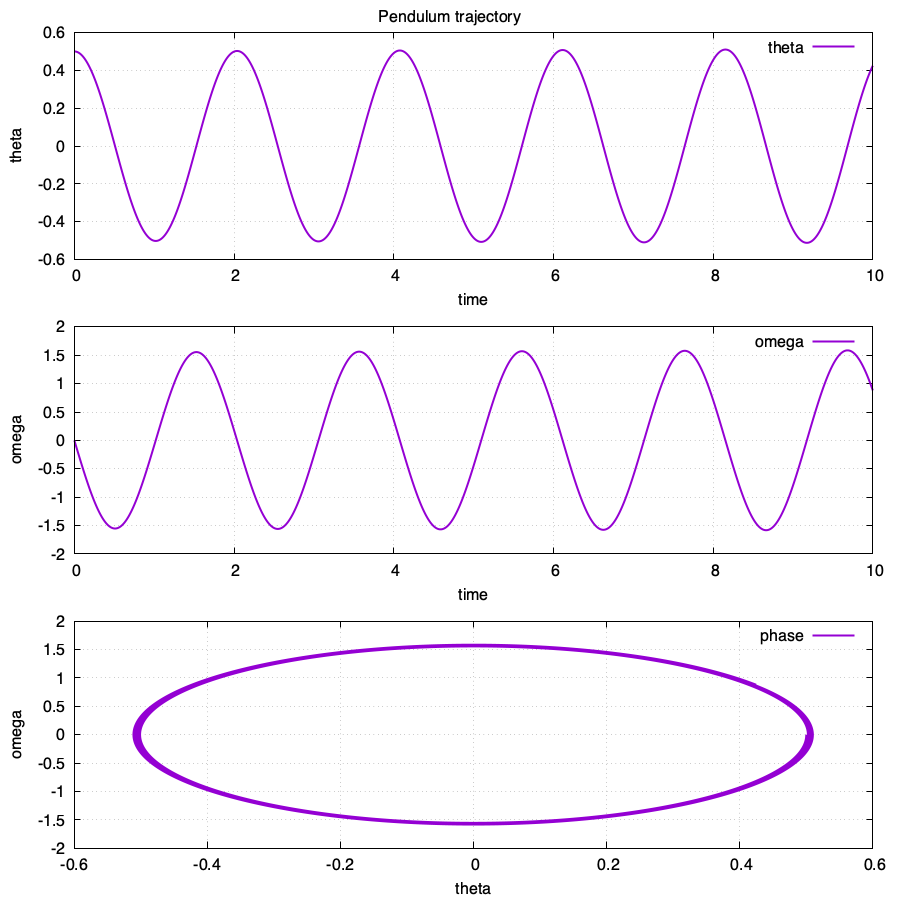
I plotted the following trajectory using GNUPlot:

(plot-trajectory (euler-solve 0.0005 (make-pendulum-ivp :theta0 15) 10.0)
                 :timestep 0.0005
                 :output-file "pendulum.png"
                 :open-file t)

The Core RK Idea

The Euler method is essentially an order-1 Taylor step. The obvious move to increase accuracy is to just keep more Taylor terms to get higher order. However, getting those higher terms are very expensive, because you have to differentiate multiple times. You must symbolically compute and code up all these partial derivatives of $f$.

The core idea for Runge-Kutta is that we can get the same level of accuracy, using only $f$ itself. You can match those Taylor terms without ever computing a single derivative of $f$. Instead of evaluating $y''$, we evaluate $f$ at a few cleverly chosen nearby points, and take a weighted average. The differences between those evaluations secretly encode the derivative information you need.

Runge-Kutta Recipe

Fundamentally, an s-stage RK method looks very similar to the Euler method:

\begin{equation*} y_{n+1} = y_n + h \sum_{i=1}^{s} b_i k_i \end{equation*}

An s-stage RK method is fundamentally a weighted average of sampled points of the given derivative. Each $k_i$ can be calculated as such:

\begin{equation*} k_i = f\left(\underbrace{t_n + c_i h}_{t}, \underbrace{y_n + h \sum_{j=1}^{s} a_{ij} k_j}_{y}\right), \quad i=1, \dots, s \end{equation*}

- $s$ = how many slope samples you take per step - $k_i$ is the $i$-th sampled slope - $c_i$ = the node: When in the step you sample, as a fraction - $a_{ij}$ = the coupling. How much of each earlier slope $k_j$ you use to nudge the state before sampling $k_i$. - $b_i$ = the weights: how you blend all the slopes into one final step.

Each method in the family is nothing but 3 arrays: a node vector c, a weight vector b, and a coupling matrix $A = (a_{ij})$

Butcher Tableau

Because each method is just dependent on changing the two vectors and the matrix, there is a more efficient way to describe it.

\begin{equation*} \begin{array}{c|c} c & A \\ \hline & b^\top \end{array} \;=\; \begin{array}{c|ccc} c_1 & a_{11} & \cdots & a_{1s} \\ \vdots & \vdots & \ddots & \vdots \\ c_s & a_{s1} & \cdots & a_{ss} \\ \hline & b_1 & \cdots & b_s \end{array} \end{equation*}

If the A matrix is strictly lower triangular, that means each $k_i$ depends only on earlier slopes. You compute $k_1, ..., k_n$ via pure substitution. This is explicit RK.

If a k_i appears on both sides of its own equation, each step requires solving a system of linear equations. This is an implicit RK (cure to stiffness).

Euler as the tiniest tableau (s = 1)

\begin{equation*} k_1 = f(t_n, y_n), \quad y_{n+1} = y_n + h k_1, \end{equation*}

This corresponds to the following tableau:

\begin{array}{c|c} 0 & 0 \\ \hline & 1 \end{array}

Explicit midpoint method (s = 2)

If we add two scouts, we can simulate the second derivative calculation. This means it is an order 2 approximation, because the error is proportional to $O(h^3)$.

\begin{equation} \begin{aligned} k_1 &= f(t_n, y_n) & &\text{slope at start} \\ k_2 &= f\left(t_n + \frac{h}{2},\ y_n + \frac{h}{2}k_1\right) & &\text{slope at peeked midpoint} \\ y_{n+1} &= y_n + h k_2 & &\text{step using only midpoint slope} \end{aligned} \end{equation}

This is the butchers tableau:

\begin{array}{c|cc} 0 & 0 & 0 \\ \frac{1}{2} & \frac{1}{2} & 0 \\ \hline & 0 & 1 \end{array}

The tableau is extremely useful, because it abstracts away the details of RK methods into just 3 arrays.

Heun's Method in Lisp

We will be implementing Heun's Method as one example in the family of second order RK methods. This algorithm simply finds the slope of two samples, and takes the average of those two values to approximate the second derivative. Using the vectorization functions defined before:

;; Heun's method (improved Euler / predictor-corrector):
;;   k1 = f(y_n)
;;   y* = y_n + dt * k1
;;   k2 = f(y*)
;;   y_{n+1} = y_n + (dt/2) * (k1 + k2)

(defun heun-step (timestep ivpair)
  (let* ((yn (ivp-initial-state ivpair))
         (ode (ivp-ode ivpair))
         (k1 (funcall ode yn))
         (k2 (funcall ode (vec-add yn (vec-scale timestep k1))))
         (new-ivp (copy-ivp ivpair)))
    (setf (ivp-initial-state new-ivp)
          (vec-add yn (vec-scale (* 0.5 timestep) (vec-add k1 k2))))
    new-ivp))

(defun heun-solve (timestep ivpair time)
  (let ((num-timesteps (floor (/ time timestep))))
    (loop for i from 0 to num-timesteps
          for current = ivpair then (heun-step timestep current)
          collect (ivp-initial-state current))))

The slope is evaluated at 2 points, first the current $y_n$ and then the euler calculated $y_{n + 1}$. That slope is averaged out, and treated as the slope for the next timestep. This slope is theoretically more accurate than just the single slope from $y_n$ or $y_{n+1}$. Because we use both slopes and average them out, the second derivative information is automatically encoded in the next step.

The plot looks like this:


(plot-trajectory (heun-solve 0.005 (make-pendulum-ivp :theta0 15) 10.0)
                 :timestep 0.005
                 :output-file "images/heun-pendulum.png"
                 :open-file t)